The Cross-Section of Volatility and Expected Returns
Andrew Ang, Robert J. Hodrick, Yuhang Xing, Xiaoyan Zhang. "The Cross-Section of Volatility and Expected Returns." Journal of Finance (2006): 259-299.
In this paper, the authors seek to examine the effects of aggregate volatility on the cross section of stock returns. They hypothesize that while the time-series relation of volatility and expected market return has been thoroughly researched, further consideration with respect to the cross section of stock returns should show that the volatility of the market return is a systematic risk factor and should be priced in the cross section of stock returns. With this, they then suggest that stocks with different sensitivities to aggregate volatility innovations should have different expected returns. To test this hypothesis, the authors look to show whether the aggregate market volatility is a priced risk factor and, if so, determine the price of this factor. They also examine the cross-sectional relationship between idiosyncratic volatility and expected returns to test whether such a risk factor is orthogonal to existing factors.
Theoretical Motivation
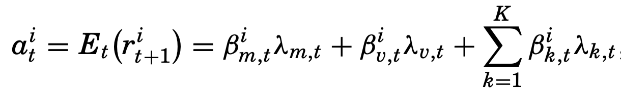
The model that they look to test is of the following form,
where (in order from left to right) the loading on the excess market return, asset sensitivity to volatility risk, and loadings of K other factors are regressed on excess stock returns.
They then simplify the above to arrive at the following with respect to expected returns,
Empirical Test
Because we do not yet know the true set of risk factors and, as a result, cannot observe such loadings of factors, the authors design a practical empirical framework to test their hypothesis.
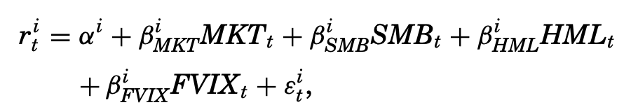
As a measure of innovations in aggregate volatility, the authors use daily changes in the VIX index. This is represented in their pre-formation regression,
which is used to test the difference in average returns of stocks with different sensitivities to innovations in aggregate volatility. Quintile portfolios are made by sorting from lowest to highest the regressed results of the loadings on the volatility factor. The stocks of each portfolio are then value-weighted. They measure the difference of average returns between portfolios with the highest and lowest volatility coefficients and find a difference of -1.04% per month that is statistically significant at the 1% level. This can be seen in the mean column of Table 1 below,
Factor Risk Explanation
The authors then look to create a factor from aggregate volatility innovations to suggest a factor risk-based explanation for the above results. This factor, called FVIX, is then used to measure ex post exposure to aggregate volatility risk. The following regression is used for the creation of FVIX by estimating the coefficient of the returns on the base assets X,
where the previous quintile portfolios are used for the base assets.
After constructing FVIX, the authors then substitute FVIX for the daily change in VIX in their pre-formation regression to get the following cross-sectional regression,
however, to test this model a contemporaneous relationship between factor loadings and average returns must be shown. The authors do this by observing that the pre-formation FVIX factor loadings and pre-formation VIX factor loadings are very similar. This can be seen in the second panel of Table 1 as follows,
Post-formation factor loadings are also shown in Table 1. It is the full sample post-formation FVIX betas that are then used to examine ex post factor exposure to aggregate volatility risk. To control for market, size, and value factors from the Fama French 3 Factor model, the authors use the following regression,
From Table 1, it can be seen that the full sample post-formation loadings on FVIX are significantly different across the quintile portfolios.
Pricing Aggregate Volatility Risk
The full regression specification used to estimate the unconditional price of the aggregate volatility risk fact is as follows,
which includes momentum and liquidity factors UMD and LIQ, respectively.
The Fama-MacBeth regression results of the above are,
Regression I from above shows the estimated price of volatility risk is -0.08% per month. The effects of volatility can be measured by multiplying the -0.08 from above with the 13.13 ex post spread in FVIX betas from Table 1. This results in a difference in average returns of -1.05%, which is almost the same as the -1.04% difference in the raw average returns, suggesting the difference in raw average returns can be attributed to exposure to aggregate volatility risk.
Idiosyncratic Volatility
The authors then sort portfolios by idiosyncratic volatility to observe its effects on cross-sectional average returns. They define idiosyncratic volatility relative to the Fama French 3 Factor model as the square root of the variance of the residual. This is to control for systematic risk, however, they also sort portfolios by total volatility. As seen by Table VI below, average returns for portfolios sorted by total volatility and idiosyncratic volatility are very similar and the difference in highest and lowest volatility portfolios are statistically significant.
Robustness tests suggest these results cannot be explained by exposures to size, book-to-market, leverage, liquidity, volume, turnover, bid-ask spreads, coskewness, or dispersion in analysts' forecasts characteristics.
Conclusion
The authors conclude that aggregate market volatility is a risk factor that can be observed in the cross-section of stock returns, and that the price of this risk factor is negative and statistically significant.
Sunday, December 22, 2019
Wednesday, December 11, 2019
Conditional Skewness in Asset Pricing Tests
By Campbell Harvey and Akhtar Siddique
The single factor CAPM has been proven not to be a reliable tool in
predicting stock returns. Because of
this, some have created factors to help explain more of the variation in stock
returns such as the SMB and HML factors created by Fama and French. Harvey and
Siddique examine the linkage between the empirical evidence on these additional
factors and systematic coskewness. Since there is considerable evidence that
returns cannot b e adequately characterized by mean and variance alone, this
leads to the inclusion of the next moment – skewness. The hypothesis is that investors will attempt
to avoid stocks that are left-skewed due to risk aversion, and these stocks
should command higher expected returns as a result.
To illustrate the relationship
between skewness and expected returns, Figure 1 shows the trade-offs between
mean, variance, and skewness. Panel B
includes the risk-free rate. Any points that are tangent to the risk-free plane
are considered efficient portfolios. The
figure shows that expected return should increase as variance and skewness
increase. Also, the portfolios that are
tangent to the risk-free plane are when skewness and variance are the highest.
The formula
for finding the coskewness beta is
Using these betas, Harvey and Siddique create three portfolios. The 30 percent of stocks with the most
negative coskewness fall in the S- portfolio.
The 30 percent of stocks with the most positive coskewness fall in the
S+ portfolio. Based on the hypothesis
and figure 1, the S- portfolio should have higher expected returns. They find
the average annualized spread between the returns on S- and S+ portfolios is
3.60 percent from July 1963 to December 1993.
This result is statistically significant. They compute the coskewness for a risky asset
from its beta with the spread between the returns on the S- and S+ portfolios
and call this measure BSKS.
Using the summary stats in table 1, it is apparent that coskewness plays
a role in explaining the cross section of asset returns. Table 2 shows that conditional coskewness can
explain a significant part of the variation in returns even when factors based
on size and book/market like SMB and HML are added to the asset pricing
model. There is a significant correlation
between the pricing errors of these factor models and the S- portfolio.
Table 3 shows the R-squares of
several regressions. It first shows the R-squared of the traditional CAPM and
the 3-factor model. Then it incorporates
the S- portfolio and the SKS portfolio.
Both a cross-sectional regression (CSR) approach using rolling betas and
a full-information maximum likelihood (FIML) method using constant betas are
used. Overall, when the S- or SKS
portfolio are incorporated with the CAPM or 3-factor model, the R-squared
increases. This shows that including
coskewness in the model can help explain stock returns over and above what the 3-factor
model can.
They move on to show that the
relevance of the SMB and HML factors appears to be dependent on how old the
stock is. SMB is only significant for
stocks with less than 60 months of returns.
This could be an IPO effect, where factors other than market (like SMB
and HML) may be more useful in predicting the returns on firms with a short
return history. Skewness on the other
hand, remains significant across almost all return length groups.
In table 5, Harvey and Siddique show
the momentum factors is related to systematic skewness. They consider several different definitions
of momentum where they vary the horizon (36-2, 24-2, 12-2, 6-2, and 3-2 months)
and holding period (1, 3, 6, 12, 24, and 36 months). All the portfolios in table 5 show a clear
relation between average return and skewness.
The portfolios with the higher average returns also have the more
negative skewness.
Figure 3 shows the necessity of negative skewness to have higher mean
returns when using momentum strategies. The y-axis shows the mean annualized
return from the strategy while the length of the line on the x-axis shows the
difference in skewness between the winners and losers. The negative slope of each line indicates
that in a momentum-based trading strategy, buying the winner and selling the
loser requires acceptance of substantial negative skewness.
These findings support the
hypothesis that skewness helps explain variation in asset pricing and supports
the theory that having negative skewness should command higher abnormal returns
because investors will naturally avoid those assets because of risk
aversion. Overall, coskewness provides
us with some insight into why variables like size and book-to-market value are
important and that the momentum effect is related to systematic skewness. Harvey and Siddique concede that measurement
of ex ante skewness may be difficult due to data limitations.
Thursday, November 14, 2019
Does Corporate Headquarters Location Matter for Stock Returns?
Pirinsky, C., Wang, Q. “Does corporate headquarters locating matter for stock returns?” Journal of Finance 61.4 (2006): 1991-2015. (link)
This paper explores the connection between corporate headquarter location and stock comovement. The authors find that stocks in the same region demonstrate comovement with each other that is not explained by the general market or industry comovement. Furthermore, companies that move their headquarters show less stock comovement with companies in the previous location and greater comovement with those in the new location. This comovement could be the result of either local fundamental factors or geographic segmentation of investors. The paper tests and finds evidence against the idea that stock comovement is determined by local economic conditions and instead argues in favor of geographic investor segmentation.
The paper considers the location of a firm to be the location of its headquarters since firms often choose to locate their headquarters in a region that is close to their main operations. Of 272 Metropolitan Statistical Areas (MSA) used to define location, about 90 have at least five publicly traded companies over the sample period of 1988 to 2002. This set of MSAs is used in the empirical tests.
To measure a stocks comovement with other stocks in the same MSA the authors construct equal weighted portfolios for each MSA. They then regress the excess returns of each stock on the return of this local portfolio, $R_i^{LOC}$, (excluding the stock used as the dependent variable) and on the market factor.
\[ R_{t} = \alpha_i + \beta^{LOC}R_i^{LOC} + \beta^{MKT}R_i^{MKT} + \epsilon_{i,t} \]
This regression is also expanded to include an equal weighted industry portfolio. To address the concern that industries, as defined by CRSP, do not accurately reflect the interaction of local companies, the authors also include whichever two additional industries they find exhibit the greatest comovement with the returns of the particular stock in the regression.
\[ R_{t} = \alpha_i + \beta^{LOC}R_i^{LOC} + \beta^{MKT}R_i^{MKT} + \beta^{IND}R_i^{IND} + \sum_{K=1}^{2} \beta^{IND_K}R_i^{IND_K} + \epsilon_{i,t} \]
Table 2 presents the results from three regressions over the full sample and two sub-periods. The location beta is positive and statistically significant across all periods and regressions. Although including industry returns decreases the magnitude of the location beta, stocks continue to exhibit significant comovement with local portfolios. When additional industries are included, which are independently correlated with the stock movement, their betas are found to be negative, adding to the strength of the local comovement result.
Next, they identify 118 firms that relocate their headquarters during the period 1992-1997. Many of these firms are small and cite reasons for relocation such as moving closer to customers or the means of production. The following regression is run for the five years before and after the relocation, not including the year of the relocation. The returns of the old MSA’s index are represented by $R_t^{LOCO}$ and the returns of the new MSA’s index by $R_t^{LOCN}$.
\[ R_{t} = \alpha_i + \beta^{LOCO}R_i^{LOCO} + \beta^{LOCN}R_i^{LOCN} + \beta^{MKT}R_i^{MKT} + \beta^{IND}R_i^{IND} + \epsilon_{i,t} \]
As shown in table 3, the change in comovement with the old index is negative and the change in comovement with the new index is positive with both statistically significant. This holds both without the industry factor (2) or with (1). In fact, the comovement with the old index is reduced by nearly half in the five years after the move. The authors note that it is unlikely that the change in comovement is due to changes in the fundamental aspects of the firm since the firms in the sample generally did not make any changes in their production process.
The authors further test if local comovement of stock prices can be explained by local economic variables. They find no comovement in local earnings and no explanatory power in a measure of local economic fundamentals.
Finally, the paper address the cross-section of stocks to determine the relationship between common firm characteristics and local comovement. As seen in table 7, size, return on asset (ROA), and institutional ownership are all negatively and generally significantly correlated with comovement throughout the full sample and three sub-periods. The interpretation is that smaller stocks, as well as less profitable stocks and stocks with more individual ownership experience greater local comovement.
Given the lack of evidence for comovement of local fundamentals, as well as the finding that comovement is stronger for small firms with greater individual investor ownership, the authors suggest local comovement is due to geographic segmentation. This indicates that geographic diversification is an important consideration. However the finding that investors’ biases contribute to the local comovement effect indicates a general lack of geographic diversification. The authors conclude by noting that geographic diversity could play an important role in pension plans and 401(k) accounts.
This paper explores the connection between corporate headquarter location and stock comovement. The authors find that stocks in the same region demonstrate comovement with each other that is not explained by the general market or industry comovement. Furthermore, companies that move their headquarters show less stock comovement with companies in the previous location and greater comovement with those in the new location. This comovement could be the result of either local fundamental factors or geographic segmentation of investors. The paper tests and finds evidence against the idea that stock comovement is determined by local economic conditions and instead argues in favor of geographic investor segmentation.
The paper considers the location of a firm to be the location of its headquarters since firms often choose to locate their headquarters in a region that is close to their main operations. Of 272 Metropolitan Statistical Areas (MSA) used to define location, about 90 have at least five publicly traded companies over the sample period of 1988 to 2002. This set of MSAs is used in the empirical tests.
To measure a stocks comovement with other stocks in the same MSA the authors construct equal weighted portfolios for each MSA. They then regress the excess returns of each stock on the return of this local portfolio, $R_i^{LOC}$, (excluding the stock used as the dependent variable) and on the market factor.
\[ R_{t} = \alpha_i + \beta^{LOC}R_i^{LOC} + \beta^{MKT}R_i^{MKT} + \epsilon_{i,t} \]
This regression is also expanded to include an equal weighted industry portfolio. To address the concern that industries, as defined by CRSP, do not accurately reflect the interaction of local companies, the authors also include whichever two additional industries they find exhibit the greatest comovement with the returns of the particular stock in the regression.
\[ R_{t} = \alpha_i + \beta^{LOC}R_i^{LOC} + \beta^{MKT}R_i^{MKT} + \beta^{IND}R_i^{IND} + \sum_{K=1}^{2} \beta^{IND_K}R_i^{IND_K} + \epsilon_{i,t} \]
Table 2 presents the results from three regressions over the full sample and two sub-periods. The location beta is positive and statistically significant across all periods and regressions. Although including industry returns decreases the magnitude of the location beta, stocks continue to exhibit significant comovement with local portfolios. When additional industries are included, which are independently correlated with the stock movement, their betas are found to be negative, adding to the strength of the local comovement result.
Table 2 |
Next, they identify 118 firms that relocate their headquarters during the period 1992-1997. Many of these firms are small and cite reasons for relocation such as moving closer to customers or the means of production. The following regression is run for the five years before and after the relocation, not including the year of the relocation. The returns of the old MSA’s index are represented by $R_t^{LOCO}$ and the returns of the new MSA’s index by $R_t^{LOCN}$.
\[ R_{t} = \alpha_i + \beta^{LOCO}R_i^{LOCO} + \beta^{LOCN}R_i^{LOCN} + \beta^{MKT}R_i^{MKT} + \beta^{IND}R_i^{IND} + \epsilon_{i,t} \]
As shown in table 3, the change in comovement with the old index is negative and the change in comovement with the new index is positive with both statistically significant. This holds both without the industry factor (2) or with (1). In fact, the comovement with the old index is reduced by nearly half in the five years after the move. The authors note that it is unlikely that the change in comovement is due to changes in the fundamental aspects of the firm since the firms in the sample generally did not make any changes in their production process.
Table 3 |
The authors further test if local comovement of stock prices can be explained by local economic variables. They find no comovement in local earnings and no explanatory power in a measure of local economic fundamentals.
Finally, the paper address the cross-section of stocks to determine the relationship between common firm characteristics and local comovement. As seen in table 7, size, return on asset (ROA), and institutional ownership are all negatively and generally significantly correlated with comovement throughout the full sample and three sub-periods. The interpretation is that smaller stocks, as well as less profitable stocks and stocks with more individual ownership experience greater local comovement.
Table 7 |
Given the lack of evidence for comovement of local fundamentals, as well as the finding that comovement is stronger for small firms with greater individual investor ownership, the authors suggest local comovement is due to geographic segmentation. This indicates that geographic diversification is an important consideration. However the finding that investors’ biases contribute to the local comovement effect indicates a general lack of geographic diversification. The authors conclude by noting that geographic diversity could play an important role in pension plans and 401(k) accounts.
Price-based Return Co-movement.
Green, T.C. and Hwang,
B.H., 2009. Price-based return co-movement. Journal of Financial
Economics, 93(1), pp.37-50.
Research Question and General Results:
The paper documents a source of return co-movement
related to stock price. Specifically, stocks correlate with their counterparts
in the same price category. Using the stock-split setting and extending the
result to all stocks, authors find that stocks experiencing splits positively
co-move with low-priced stocks and negatively co-move with high-priced stocks.
Since the price-based co-movement is not germane to various firm
characteristics, authors conclude that investors categorize securities based on
their prices.
Empirical Results:
Stock-split serves a relatively clean circumstance for
evaluating the price-based co-movement. It decreases a stock’s nominal prices
without altering its firm fundamentals. In this paper, authors concentrate on
2-for-1 stock splits and construct corresponding low and high price indices. In
the stock-split setting (a decrease in a stock’s nominal price), beta
coefficients on low-priced index and high-price index are significantly
positive and negative, respectively. This result suggests that a decrease in a stock’s
nominal price by its split makes it become more correlated with its low-priced stocks
and less with high-priced stocks. Besides, authors find a similar result for
all stocks that stocks have an increased co-movement with their counterparts in
the same price category. The result is robust to common variations in industry,
firm size, transaction cost, and return momentum.
Determinants of Price-based Return
Co-movement:
The empirical results demonstrate investors categorize
stocks given their prices. Thus, authors conjecture that investors adopt price
a naïve proxy for firm size and expect more upside potentials in low-priced
stocks. The empirical test also confirms behavioral explanations. The weak
relation between institutional ownership and price-based co-movement indicate
that the co-movement is hardly driven by market frictions.
Friday, November 8, 2019
Volatility-Managed Portfolios
Moreira, Alan and Tyler Muir.
“Volatility-Managed Portfolios” The Journal of Finance Vol. 72 No. 4 (2017) 1611-16430.
“There is little relation between lagged volatility
and average returns but there is a strong relationship between lagged
volatility and current volatility.” The authors exploit this relationship to
show that significant gains can be made through volatility timing. Using last
month’s realized variance as a proxy for a portfolio’s conditional variance, they
show that, whatever the desired exposure to a variety of different portfolios,
Sharpe ratios can be improved by levering down the exposure when last month’s volatility
is high and levering up the exposure when last month’s volatility is low. They
determine volatility-managed portfolio exposure (LHS of the equation) through
weighting by the inverse of the previous month’s realized variance (RHS of the
equation).
There is a constant, c, which is chosen by the
authors to set the unconditional standard deviations of the managed and
buy-and-hold portfolios equal, but it does not influence the Sharpe ratio of
the managed portfolio.
Managed vs. Original Portfolio:
Here they regress the returns of the managed
portfolio on those of the original portfolio. Positive alpha indicates an
improvement in the Sharpe ratio. Of the chosen portfolios, only SMB and CMA
from Fama and French show no significant improvement at least at the 10% level.
When regressing managed portfolio returns on the Fama-French three factor
model, the currency carry trade joins SMB and CMA as insignificant but the rest
still show positive and significant alpha.
Expanding the Mean-Variance Frontier:
The authors use different factor models which have
been shown to be effective in explaining the cross-section of stock return to
construct in-sample mean-variance efficient portfolios. That is, for each model
considered they find the combination of factors which produces the largest Sharpe
ratio. They then run similar analysis as with the individual factors. Here, however,
a positive and significant alpha also indicates an overall expansion of the
mean-variance frontier. For each model considered, volatility-managed
mean-variance efficient portfolios show significant improvement. They also show
similar results for sub-sample analysis.
Utility Gains in the Presence of Leverage
Constraints:
Relative to a risk-averse investor’s desired exposure
to the market return, the authors also show here that for each desired exposure
considered (x-axis) there is a positive improvement to the utility of the
investor using volatility-managed portfolios even when there are leverage
constraints. They consider leverage constraints at 1.5 times (consistent with a
50% margin requirement) and 1 times the portfolio. That is, the volatility
managed exposure cannot exceed 1.5 or 1 times the market, respectively. This
indicates that there are implementable utility gains for mean-variance investors.
Wednesday, November 6, 2019
Macro-Finance
John H. Cochrane. "Macro-Finance." Review of Finance (2017): 945-985.
The author discusses different macro-finance models. He contrasts their strengths and weaknesses, suggests paths for further research, and even describes their potential in furthering macroeconomic research related to recessions.
To sample from the different preferences and market structures, he considers ten cases:
- Habits
- Recursive Utility
- Long-run risks
- Idiosyncratic risk
- Heterogeneous preferences
- Rare disasters
- Utility non separable across goods
- Leverage; balance sheet; institutional finance
- Ambiguity aversion, min-max preferences
- Behavioral finance; probability mistakes
where C is consumption, gamma is the risk aversion coefficient, and Y represents additional risk.
In each case the author describes the central idea being that the market fears recessions as well as assets with decreasing values during recessions, and that the market's risk-bearing capacity falls during recessions as a result. Each case differentiates from the rest with respect to the exact state variable for expected returns including consumption related to recent values, news regarding long-run future consumption, cross-sectional risk, or leverage. The author reasons that these state variables are highly correlated and that each resulting model has helped to describe the same underlying idea of risk perceptions and how these perceptions relate to falling investments as well as our understanding of the mismatch between the riskiness of investment projects and the higher risk aversion of those who save. It is also noted, of course, that no model has succeeded in fully describing the equity premium/risk free rate puzzle as well as the excess volatility and business cycle risk premium.
Of the cases, particularly motivating is the idiosyncratic risk model. This model is similarly represented with a discount factor and a state variable,
with y representing the cross sectional variance of individual consumption growth. It's simplicity comes from the need to only assume a cross sectional variance process (y of t+1), however, this process must satisfy certain constraints for return predictability due to the model's simplicity. The volatility of cross sectional consumption must be large and vary greatly over time (as well as at the right times). While this isn't necessarily intuitive (empirical results aren't encouraging), the solution is to have a variance of future consumption that varies over time, or as the author states, "time variation in the conditional variance of the conditional variance of cross sectional risks". This has been explored, as in Constantinides and Ghosh (2017), with further opportunities for research relating to appropriate time-varying moments in micro data. Still, the model represents a simple explanation that people fear times of large idiosyncratic consumption risk (i.e. recessions) and this exacerbates a fear of poorly performing assets during these times. The author suggests this is in line with the reasoning of the other models discussed, with differences (such as the state variable being exogenous and requiring special assumptions) boiling down to esthetic preference of the researcher.
The author concludes by advocating for the consideration of macro-finance models and their potential usefulness in macroeconomic research related to recessions. He believes that research relating to macro-finance models may help to lessen the divide between macroeconomics and macro-finance due to the strong relationship between recessions and risk premiums, risk aversion, risk-bearing capacity among investors, as well as the shift to assets perceived safe during recessions. It will be our understanding of how risk perceptions affect investors, and not risk-free interest rates or inter-temporal substitution, that allow us to better understand recessions.
Sunday, November 3, 2019
A Survey of Behavioral Finance
By: Nicholas Barberis and Richard Thaler
Barberis
and Thaler discuss the results of the behavioral finance, a fairly new field of
finance compared to the traditional finance paradigm. The key difference between behavioral finance
and the traditional finance paradigm is rationality. The traditional finance paradigm assumes
rational individuals. Rationality means
two things. First, when presented with
new information, agents update their beliefs accordingly. Second, given their beliefs, agents make
choices that are normatively acceptable.
Behavioral finance considers when some agents are not rational. Specifically, when one of the two tenets of
rationality are relaxed.
One of the
two building blocks of behavior finance is limits to arbitrage. A classic objection to behavioral finance is
that when some agents don’t act rationally, the agents who do act rationally
will prevent them from influencing prices for long due to arbitrage. A series of theoretical papers suggests
otherwise, showing that in an economy where rational and irrational investors
interact, irrationality can have a long and substantial impact on prices. This stands counter to the efficient markets
hypothesis (EMH), where put simply, the “prices are right.” Limits to arbitrage
suggest that mispricing does occur and can persist. Some reasons these limits exist are the
fundamental risks the arbitrageur faces, noise trader risks, and implementation
costs. Some evidence of the limits to
arbitrage are twin shares, index inclusions, and internet carve-outs.
The other
building block of behavior finance is psychology. The theory of limited arbitrage shows
irrational traders can cause deviations from fundamental value, but psychology seeks
to tell us why those traders act irrationally.
For guidance, economists consider extensive evidence compiled by
cognitive psychologists on the systematic biases that arise when people form
beliefs, and on people’s preferences.
Some of these beliefs that are particularly useful to behavioral finance
are overconfidence, optimism and wishful thinking, representativeness,
conservatism, belief perseverance, and anchoring. A couple things to focus on when considering
preferences are prospect theory and ambiguity aversion.
Barberis
and Thaler follow this overview by explaining some applications of behavioral finance. The first is the aggregate stock market,
where behavioral finance may help solve the equity premium puzzle and the
volatility puzzle. The second is the
cross-section of average returns.
Behavioral finance may help explain some anomalies, such as the size
premium, long-term reversals, the predictive power of scaled-price ratios,
momentum, and event studies of earnings announcements, dividend initiations and
omissions, stock repurchases, and primary and secondary offerings. The third application is closed-end funds and
comovement. The fourth is investor behavior
where irrationality and psychology can explain insufficient diversification, naïve
diversification, excessive trading, the selling decision, and the buying
decision. The last application mentioned
is corporate finance, where behavioral finance can address security issuance,
capital structure, investment, and dividends.
When De
Bondt and Thaler (1985) published their paper, many scholars felt the best explanation
was programming error. Since then, most
of the empirical facts are agreed upon but the interpretation of those facts in
still in dispute. Behavioral finance has
been very helpful in understanding possible limits of arbitrage and bounded
rationality. Barberis and Thaler concede
there are numerous degrees of freedom but note that rational modelers have just
as many options to choose from. There is
only one scientific way to compare alternative theories, behavioral or
rational, and that is with empirical tests. They say we should be skeptical of theories
based on behavior that is undocumented empirically. Barberis and Thaler conclude by giving two
predictions. First, we will find out
that most of our current theories, both rational and behavioral, are
wrong. Second, substantially better
theories will emerge.
Thursday, October 31, 2019
Empirical Cross-Sectional Asset Pricing
Stefan Nagel. “Empirical
Cross-Sectional Asset Pricing” The Annual Review of Financial Economics (2013) 5:167-199.
The author reviews research in
several aspects of empirical cross-sectional asset pricing. Other posts here have
and will highlight papers which touch on some of them, so I summarize only a
couple of general themes.
There are approaches to
cross-sectional asset pricing which distinguish explanations for why investors
price assets the way they do and approaches which do not. “The economic content
of pricing models is … in the restrictions that they impose on the [stochastic
discount factor].” Ad hoc factor models and production-based models, while
useful in cross-sectional tests, do not rely on investor preferences for their
restrictions on the SDF and, so, do not explain the “why”. Rational
(consumption-based, long-run risk) as well as sentiment-based tests based on
theoretical restrictions on investor preferences give them a higher degree of
economic content. Frictions and liquidity risk can cause rational models to fail,
but studies in these areas provide evidence for “why” assets are priced the way
they are. That is, additional risks exist for which investors rationally
require additional return in order to bear the risk.
A significant amount of
cross-sectional asset pricing research is centered around finding deviations from
accepted models (anomalies). Recent studies have urged caution in this pursuit,
however. The possibility for data snooping, where some spurious anomalies are
randomly found to be significant, is an ever-present problem. Adjusting
critical values and performing out-of-sample testing are ways suggested in the
literature to help attenuate the problem. However, the author notes that pseudo
out-of-sample testing is not necessarily a solution because data can be mined
to find significant result here as well. True out-of-sample testing is
necessary to lend validation to results. A true out-of-sample test occurs when
data is used that was not available or used for the original study. Some ways
this has been done in the literature is the use of data from different markets,
post-publication data of the same asset(s) used in the original study, and in
some cases even pre-sample data that became available after publication. It has
additionally been found that use of r-squared statistics as an indication of how
well a model or factor explain the cross-section of asset returns can be
misleading when the test assets have a low-dimensional factor structure.
Investor sentiment happens when
asset prices are evaluated under a subjective probability distribution. Its
effect on asset prices is persistent when this sentiment is correlated across
enough investors and there are significant enough risks to dissuade or prevent
sophisticated investors from taking opposite positions and driving prices back
to their fundamental values. Investor sentiment and rational explanations for
return predictability need not be mutually exclusive. Research in this area
focuses both on finding and testing empirical proxies for investor sentiment
and on investigating the limits to arbitrage preventing sophisticated investors
from correcting mispricing. Analyst forecasts, style fund returns, and mutual
fund inflows are a few examples of proxies used with some success as proxies
for investor sentiment.
Real world investors must learn about
the return generating process in real time. Therefore, return predictability
obvious to researchers in retrospect may not have been known or obvious to
investors. Out-of-sample testing on variables shown to have ability to predict
returns is one area of research into investor learning. For example, studies
have shown that there is a decay of predictability after the publication of
research about return predictors. The implication is that something not known to
real-world investors becomes known upon publication and they then move to
exploit it to the extent possible. Additional research has been done using pseudo
out-of-sample testing where early periods in the data are used as a training
sample to predict future returns. The author notes that investor learning does
not fall under rational expectations or sentiment.
Empirical cross-sectional asset
pricing research has come a long way and there is much yet to be explored. Many
avenues of research are fruitful, but the ones with the greatest economic
content are those which have something to say about the preferences of
investors because they offer insight into understanding not just what is
happening but “why” investors are pricing assets the way they are.
Subscribe to:
Posts (Atom)